
The core fallacy in HMLV planning is treating the master schedule as a deterministic forecast; true profitability comes from designing a system that thrives on unpredictability.
- Static, weekly schedules are fundamentally incompatible with the high-variability nature of bespoke electronics, actively destroying margins through data latency and inefficient capital allocation.
- Switching from traditional JIT to a Just-in-Sequence (JIS) material flow, coupled with event-driven triggers, is the key to synchronising component arrivals with real-time production cell capacity.
Recommendation: Stop attempting to perfect your forecast. Instead, focus on building an algorithmic, self-correcting system that treats lead times and capacity as probability distributions, not fixed numbers.
For any Production Planner or Operations Manager in bespoke electronics manufacturing, the scene is painfully familiar. The master production schedule, painstakingly compiled, becomes obsolete the moment it is published. An unexpected component shortage on one line, a client’s last-minute change order, or a minor machine stoppage on another creates a cascade of disruptions that no static plan can absorb. The daily reality becomes a frantic exercise in firefighting, expediting, and apologising for delays, all while cash is tied up in components that aren’t needed and margins are silently eroded.
The conventional wisdom offers familiar but ultimately inadequate solutions: foster better supplier relationships, hold more safety stock, or conduct more frequent planning meetings. While not without merit, these actions treat the symptoms, not the underlying disease. They are attempts to reinforce a planning paradigm that is fundamentally broken in a High-Mix, Low-Volume (HMLV) environment. The constant variability is not a problem to be solved; it is the inherent nature of the business.
But what if the entire concept of a fixed, forward-looking master schedule is the root of the failure? What if true operational control comes not from attempting to predict the future with greater accuracy, but from building a system with the algorithmic reflexes to react to the present, instantly? This requires a paradigm shift: from forecasting to responding, from static commands to dynamic synchronisation. It is a move towards a system where material flow is not just « just-in-time » but precisely sequenced and algorithmically coupled to real-time events on the factory floor.
This article deconstructs the core technical and strategic shifts required for this transformation. We will dissect the failures of traditional MRP in HMLV, provide a blueprint for algorithmic material synchronisation, and detail the data-driven models needed to correct the planning fallacies that quietly destroy profitability. This is not about better planning; it is about a better system of planning.
Contents: A Guide to Algorithmic MRP Optimisation
- Why Static Planning Paradigms Destroy Margins on Bespoke Component Orders?
- How to Synchronise Material Arrivals With Dynamic Production Cell Capacities?
- Daily Micro-Adjustments vs Weekly Master Schedules: What Minimises Downtime?
- The Safety Stock Assumption That Leads to Massive Microchip Inventory Obsolescence
- Correcting Lead Time Inaccuracies That Consistently Delay Client Deliveries
- Automating Reorder Points to Prevent Accidental Overstocking
- The Micro-Stop Ignorance That Quietly Steals 15% of Daily Capacity
- Maximising Overall Equipment Effectiveness in Food and Beverage Processing
Why Static Planning Paradigms Destroy Margins on Bespoke Component Orders?
The fundamental flaw of static planning—typified by the weekly or bi-weekly Master Production Schedule (MPS) refresh—is its inherent latency. In an HMLV environment where every order can be unique, the plan is a snapshot of a reality that has already changed. This time lag between data collection, plan generation, and execution creates a significant, often unmeasured, data latency cost. This cost manifests as premium freight charges for expedited components, line-down time waiting for a missing part that the system thought was in stock, and the capital cost of holding inventory that was ordered based on a now-irrelevant forecast.
Static paradigms operate on assumptions of stability that simply do not exist in bespoke assembly. They assume lead times are fixed, yields are predictable, and customer demand is stable for the duration of the planning cycle. Each of these assumptions is a point of failure. The system’s inability to react in real-time to a machine failure, a quality issue with a batch of components, or a sudden change in cell capacity means that by the time the next planning cycle begins, the operation is already dealing with the costly consequences of the previous plan’s inaccuracies.
Case Study: The Impact of Dynamic Frameworks
The transition to a dynamic system yields quantifiable results. For instance, a high-mix, low-volume ship parts supplier, facing similar challenges of custom orders, implemented a digital twin-enhanced framework for real-time planning. The results were a 27% improvement in daily output and a 21% reduction in manufacturing cycle time, demonstrating a direct correlation between reducing planning latency and boosting operational efficiency.
This is not a failure of the planners; it is a failure of the tools and paradigms. The attempt to force the chaotic reality of HMLV into the rigid structure of a static plan is the primary source of margin erosion. The goal should not be to create a more accurate static plan, but to eliminate the static nature of the plan itself.
How to Synchronise Material Arrivals With Dynamic Production Cell Capacities?
The solution to static plan failure is not merely faster planning, but a fundamental shift in how material flow is conceived and executed. The objective is material synchronisation: the perfect, dynamic alignment of component delivery with the real-time consumption needs of a specific work order at a specific production cell. This moves beyond traditional Just-in-Time (JIT) to a more granular, precise model: Just-in-Sequence (JIS).
This image provides a macro view of what JIS looks like in practice: components are not just delivered ‘on time’ in bulk, but are kitted and presented in the exact sequence of consumption for a specific, unique assembly. This eliminates setup time for part searching and dramatically reduces the chance of using an incorrect component.
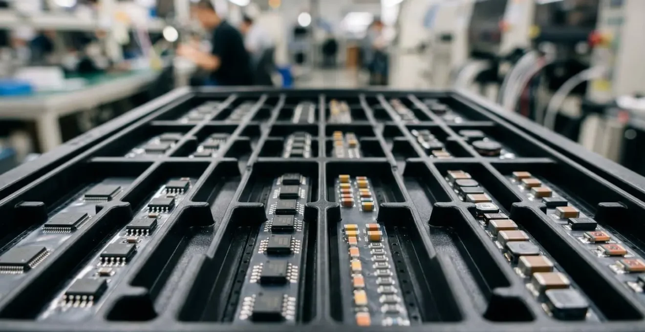
Achieving this level of synchronisation requires a deep, event-driven coupling between the Manufacturing Execution System (MES) and the MRP. When an MES signals that a work order has started at a cell, it should trigger an automated pull signal for the corresponding JIS kit. This ensures that materials arrive precisely when needed, not based on a week-old schedule. The comparison between these two approaches reveals the stark advantages of sequencing.
This table, based on comparative analysis of material flow systems, highlights the specific gains for HMLV electronics. JIS isn’t just a logistics tactic; it’s a strategic weapon that directly boosts capacity utilisation and quality by design.
| Aspect | Traditional JIT | Just-in-Sequence (JIS) | Impact on HMLV Electronics |
|---|---|---|---|
| Material Arrival | On-time for production window | Exact sequence for work order | Reduces changeover by 40% |
| Kitting Approach | Batch-based | Order-specific kits | Eliminates wrong-part errors |
| Cell Capacity Response | Static allocation | Dynamic real-time adjustment | 15% capacity utilization gain |
| MRP-MES Integration | Daily sync | Event-driven coupling | Sub-minute response time |
By synchronising material arrivals with the actual, real-time pace of production cells, you transform inventory from a liability (a buffer against a bad forecast) into a dynamic asset that flows in perfect harmony with value creation.
Daily Micro-Adjustments vs Weekly Master Schedules: What Minimises Downtime?
The debate between rigid weekly schedules and fluid daily adjustments is at the heart of the HMLV challenge. A weekly master schedule provides a sense of stability and long-term visibility, but it is a brittle stability that shatters upon contact with reality. Daily micro-adjustments, driven by real-time data, create a system that is antifragile—it gains strength from volatility. The key is to shift the planning mindset from setting fixed output rates to maintaining a consistent production rhythm.
In this model, concepts like Takt compliance become paramount. It’s not about hitting a rigid daily target of X units, which is often impossible with varying order complexities. Instead, it’s about the planning system’s ability to maintain a steady flow and rhythm, adjusting resource and material allocation in real-time to smooth out bottlenecks before they cause a line-down situation. This is where weekly schedules fail catastrophically; a problem that occurs on Monday might not even be visible to the planning system until the next weekly review, by which time hours of capacity have been lost.
A system built for daily micro-adjustments leverages continuous feedback loops. An automated alert that a critical machine’s output has dropped by 5% in the last hour doesn’t just trigger a maintenance call; it also triggers the MRP to recalculate the capacity for the next 24 hours and potentially re-route an upcoming order to a different cell. This is algorithmic, real-time problem-solving, not reactive firefighting. As research on production flexibility shows that changeover time and first-pass yield are the true north stars, a system that can make intelligent, data-driven adjustments on an hourly or daily basis will always outperform one that is locked into a weekly plan.
The goal is to minimise the « time to detect » and « time to react » for any deviation from the plan. A weekly schedule has a time-to-react measured in days. A dynamic system has a time-to-react measured in minutes or seconds. In the competitive landscape of bespoke electronics, that difference is the line between profit and loss.
The Safety Stock Assumption That Leads to Massive Microchip Inventory Obsolescence
The traditional safety stock formula—often a simplistic « days of supply » calculation—is one of the most dangerous assumptions in modern electronics manufacturing. It treats all components as equal and assumes the past is a reliable predictor of the future. This assumption is particularly perilous when dealing with microchips and other semiconductors, where lifecycles are short, and the market is volatile. Holding a 30-day supply of a component based on historical usage is a direct path to inventory obsolescence.
The core problem is that this method is blind to market dynamics. The electronics supply chain is in constant flux. While overall supply has improved since the crisis of 2022, the semiconductor market continues to expand rapidly. In fact, industry analysis reveals that the semiconductor industry is projected to see 16% growth in 2024 alone. This growth fuels rapid innovation, meaning the « standard » microchip in your safety stock today could be superseded by a cheaper, more powerful alternative tomorrow, rendering your inventory worthless.
The modern approach requires a shift from static safety stock to dynamic buffer management. This involves an intelligent, real-time analysis of inventory levels, not against a fixed target, but against a probabilistically calculated future demand and supply risk. An inventory specialist, armed with the right tools, should be evaluating component lifecycle data, market availability trends, and supplier reliability scores—not just counting parts on a shelf.

Instead of a flat 30-day supply, a dynamic system might recommend a 45-day buffer for a hard-to-source, sole-sourced component with a volatile lead time, while simultaneously flagging a 10-day supply of a common resistor as excessive due to high market availability and multiple qualified suppliers. This algorithmic precision releases working capital and drastically reduces the risk of being left with a warehouse full of obsolete electronics.
Correcting Lead Time Inaccuracies That Consistently Delay Client Deliveries
The single lead time figure stored in most MRP systems is a fiction. It is a single point estimate representing a complex probability distribution. Relying on this one number— »Supplier X has a 28-day lead time for part Y »—is a primary driver of missed deadlines. The reality is that the lead time might be 28 days on average, but it could range from 15 days to 50 days depending on factory capacity, raw material availability, and logistics disruptions. Planning based on the average is planning to fail.
To build a reliable schedule, one must move from using a single, fixed lead time to a probabilistic lead time model. This means the MRP system must understand not just the average, but the variance. Instead of storing « 28 days, » it should store a distribution (e.g., a normal distribution with a mean of 28 and a standard deviation of 5 days). This allows for more intelligent planning, such as calculating the 95th percentile lead time (the time within which 95% of orders will arrive) for critical path components.
The data clearly shows how volatile and component-specific these lead times are, making a single-number approach untenable. This table, based on a recent analysis of the electronic components outlook, illustrates the vast differences and ongoing volatility across component types.
| Component Type | 2022 Peak Lead Time | 2024-2025 Lead Time | Probability Distribution Benefit |
|---|---|---|---|
| Automotive MCUs | >50 weeks | 20-30 weeks | 30% accuracy improvement |
| Standard Logic | 30+ weeks | 10-15 weeks | Normalized to low double-digits |
| High-cap MLCCs | 26+ weeks | 10-26 weeks (increasing) | Better demand spike handling |
| AI Processors | N/A | On allocation | Critical for capacity planning |
Correcting this requires a systematic, data-driven approach to tracking and scoring supplier reliability. It’s not about arguing with suppliers; it’s about building a system that automatically accounts for their real-world performance. The following checklist provides a concrete framework for building such a system.
Action Plan: Building a Supplier Reliability Scoring System
- Track on-time delivery performance across all suppliers with a weighted 60-day rolling average to capture recent trends.
- Monitor quality acceptance rates, including first-pass yield at your facility and the frequency of Return Material Authorisations (RMAs).
- Integrate real-time logistics provider APIs to gain in-transit visibility and replace static ETAs with dynamic, calculated ones.
- Apply an algorithmic scoring model that automatically favours suppliers with higher reliability scores in your MRP, even at marginally higher unit costs.
- Create automated alerts that trigger a review or alternative sourcing process when a key supplier’s reliability score drops below a predefined threshold.
Automating Reorder Points to Prevent Accidental Overstocking
Static reorder points (ROPs) are the direct consequence of the flawed assumptions about safety stock and lead times. If your system believes lead time is a fixed number and demand is stable, then setting a trigger to « order more when stock falls to X units » seems logical. However, in the dynamic world of HMLV, this simple logic is a recipe for either stockouts or overstocking. A sudden spike in demand for a component will drain inventory below the ROP before the next planning cycle, leading to a shortage. Conversely, a drop in demand will leave you with excess stock ordered by an unthinking system.
The solution is the implementation of dynamic, algorithmically-driven ROPs. A dynamic ROP is not a single number but a calculated value that constantly adjusts based on real-time data inputs. These inputs include:
- Real-time consumption data: How fast is the component actually being used on the line today, not last month?
- Probabilistic lead time: The system should use the 95th percentile lead time from your supplier reliability model, not the average.
- Short-term demand forecast: What is the confirmed and projected demand for this component over its calculated lead time?
This level of real-time calculation and integration was once computationally prohibitive. However, the rise of advanced processing capabilities makes it feasible. The significant industry investment in technologies like high-speed AI network fabrics is creating the backbone necessary to support these complex, real-time calculations across an entire enterprise. This allows an MRP to continuously ask, « Based on what I know *right now*, what is the optimal point at which to reorder this specific component to balance service level against inventory cost? »
Automating this calculation prevents the accidental overstocking that occurs when planners, burned by past shortages, manually inflate ROPs « just in case. » The algorithm provides a disciplined, data-driven approach that removes emotion and guesswork from the inventory management process, directly freeing up working capital.
The Micro-Stop Ignorance That Quietly Steals 15% of Daily Capacity
While major equipment breakdowns are immediately visible and tracked, a more insidious threat to capacity goes largely unnoticed: the micro-stop. These are short-duration stoppages, typically between 30 and 120 seconds, that are too brief to be logged as official downtime by operators. An operator waiting 45 seconds for a component kit to arrive, or a machine pausing for 90 seconds while a feed is adjusted, will rarely log the event. Yet, cumulatively, thousands of these micro-stops across a facility can quietly steal upwards of 15% of total productive capacity each day.
The core issue is one of data capture. Traditional MES and ERP systems are blind to this phenomenon. Without data, the problem is invisible and therefore unsolvable. Operations managers may see that a line produced 15% fewer units than its theoretical maximum but have no data to explain why. The cause is often misattributed to « operator inefficiency » when the real culprit is a systemic failure in material flow or process stability.
The key to reclaiming this lost capacity is to make the invisible visible through Industrial Internet of Things (IIoT) technology. By implementing a system to detect these events automatically, you can begin to categorise and address their root causes. A practical approach includes:
- Deploying low-cost vibration, current, or light-curtain sensors on critical equipment to automatically detect any pause in operation longer than a set threshold (e.g., 20 seconds).
- Configuring the MES to automatically log and categorise these micro-stops based on machine state or operator input (e.g., ‘Waiting for Material’, ‘Tool Adjustment’, ‘Quality Check’).
- Creating real-time dashboards that visualise the cumulative impact of micro-stops, turning a series of minor annoyances into a significant, quantifiable financial loss.
- Linking micro-stop patterns directly back to the MRP system to identify correlations between component shortages and production pauses.
Ignoring micro-stops is equivalent to ignoring a 15% tax on your production capacity. By implementing the technology to detect and analyse them, you can uncover a massive hidden reservoir of productivity without a single pound of capital expenditure on new machinery.
Key Takeaways
- Stop trying to perfect the static schedule; it’s the root of the problem. True efficiency in HMLV comes from building a system that reacts to, rather than predicts, reality.
- Profitability is a direct function of material synchronisation. Shift your focus from basic Just-in-Time (JIT) to the more precise, order-specific model of Just-in-Sequence (JIS).
- Treat all planning variables—especially lead times and supplier performance—as probability distributions, not fixed numbers. An MRP system that understands variance is an absolute necessity.
Maximising Overall Equipment Effectiveness in Food and Beverage Processing
While this article’s focus is on HMLV electronics assembly, the discipline of Overall Equipment Effectiveness (OEE) offers universal principles. The title mentions food and beverage processing, a high-volume, low-mix industry, to make a critical point: the fundamental components of OEE—Availability, Performance, and Quality—must be radically re-interpreted for an HMLV environment. Applying high-volume OEE metrics directly to a bespoke electronics facility is a recipe for misleading data and poor decisions.
In traditional manufacturing, maximising OEE often means running one product for as long as possible at maximum speed. In HMLV electronics, this approach is disastrous. A high OEE score achieved by running a single, simple product for a full shift is meaningless if your order book is filled with complex, one-off assemblies. The definition of « good » performance must change. As the following table shows, the strategies for optimising each OEE component are starkly different.
This comparison, informed by cross-industry OEE optimisation analysis, demonstrates how HMLV must prioritise sequence and changeover efficiency over raw speed.
| OEE Component | Traditional High-Volume | HMLV Electronics Assembly | Revenue Impact |
|---|---|---|---|
| Availability | Focus on uptime | Smart changeover grouping | +12% revenue/sq ft |
| Performance | Speed optimization | Sequence optimization | Reduced setup by 40% |
| Quality | End-product inspection | Real-time AOI integration | First-pass yield +15% |
The ultimate goal in HMLV is not maximum OEE, but maximum profitable throughput. This means optimising the entire system—from material planning to production sequencing—to maximise revenue generated per square foot of factory space. As modern case studies show, this is achieved when AI-driven planning and digital supply chains are fully integrated. An intelligent system doesn’t just schedule production; it analyses demand, optimises sequences to minimise changeovers, and proactively suggests alternative materials when it detects a potential supply chain disruption. This holistic, algorithmic approach is what transforms HMLV from a chaotic challenge into a scalable, competitive advantage.
The transition from a static, forecast-driven MRP to a dynamic, algorithmically-synchronised system is not merely a software upgrade; it is a fundamental shift in operational philosophy. The first and most critical step on this journey is to begin measuring the true cost of your data latency. Evaluate your current processes today to identify where outdated information is driving poor decisions and eroding your margins.